LibreOffice Calc functions to make your work easier

LibreOffice is an outstanding open source office suite. I especially love the LibreOffice Calc spreadsheet, which is a powerful alternative to proprietary spreadsheets.

I find all kinds of uses for spreadsheets. As an undergraduate physics student, years ago, I relied on spreadsheets every day to analyze lab data. Today, I use spreadsheets for all kinds of things. I’m a consultant, and I use spreadsheets to track my budget and expenses. I teach university courses, and I use spreadsheets to calculate and assign grades. I also use spreadsheets to plan major purchases.

If you know the right function to apply, spreadsheets like LibreOffice Calc make it easy to analyze and reduce data. Here are the LibreOffice Calc functions that I use all the time to get my work done.

Columns and rows

Before I show the functions I use the most, it might help to start with a few notes about how spreadsheets track data.

All spreadsheets since the days of VisiCalc (1979) use letters for columns and numbers for rows. You address each cell with a combination of a letter and number, such as A1 for the cell in column A and row 1.

To specify a range of values, you need to give the cell address for the start and end of the range. For example, to indicate the first 5 cells in the first two columns, you would write A1:B5 because the “upper left” end of the range starts in cell A1 and the range ends in the “lower right” in cell B5.

If I’m going to work on data in rows and columns, I’ll use AutoFill to repeat a calculation into adjacent cells. For example, I might have a set of values in column A, and I want to perform calculations with those numbers in column B. For B1, I might use =A1*2 to double the value. “Dragging” the block in the lower-right corner of B1 allows me to use AutoFill to do the same calculation for each cell in column B.

But to reference a range of values, I might not want AutoFill to “translate” these references for me. That’s when I find it helpful to “lock off” a column or row reference with the $ prefix operator. For example, to always access the range A1:B5, even when using AutoFill, I can “lock” the row references with $ like A$1:B$5 so AutoFill will continue to access the same range when filling to adjacent rows. To “lock” column references, use $ before the column reference, such as $A1:$B5 so AutoFill will access the same range when filling to adjacent columns.

You can also use named ranges, but I find the $ is enough for most of what I do in spreadsheets. You’ll see this come up in several of my examples.

Basic calculations

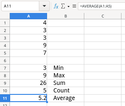
I use these basic functions the most to analyze data. The MIN function returns the smallest value in a range; similarly, the MAX function returns the largest value. You can use SUM to add the values in a range, and COUNT to return the number of items in a range. In theory, you could divide SUM by COUNT to get the average, but it’s easier and more reliable to use AVERAGE.

Applying conditions

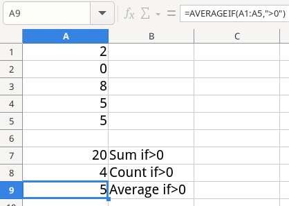
Sometimes, it’s helpful to perform a calculation on a range while ignoring certain data. That’s when these “If” functions become super useful. SUMIF adds the values in a range, depending on a condition. COUNTIF will count the items, depending on a condition. And AVERAGEIF calculates the average, depending on a condition.

You enter the range as you would with SUM or COUNT or AVERAGE, and provide the condition in quotes. For example, if you only wanted to consider values above zero, enter ">0" for the condition.

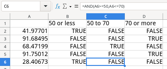
At other times, you might only need to compare a value. That’s where the logical functions become useful. The IF function performs a test and returns a true or false value. For example, =IF(A1>0) returns TRUE if the value in cell A1 is a number that’s greater than zero, and FALSE otherwise.

You can combine tests with the AND and OR functions. These are functions, not operators. That means you can’t combine comparisons with AND; instead, you need to use AND as a function. Include each test as separate function arguments.

Random numbers

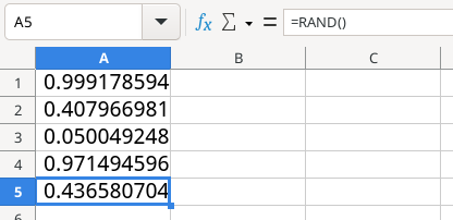
Spreadsheets help to model data. But data doesn’t have to be static, you can provide a “fuzz factor” by introducing a random value. Use the RAND function to generate a random number from 0 to 1, although the random number never quite gets to 1. The random number will change every time you update the spreadsheet, such as entering data in a new cell.

Rounding numbers

When I model random values using RAND, I usually multiply the random number by some other number to get a random value in a range, such as =RAND()*10 to get a number from 1 to 10. At the same time, I usually don’t want the stuff after the decimal point. For that, I need to cut off the extra digits.

Spreadsheets provide two handy functions to do that: INT will return just the number before the decimal point, creating an integer value. ROUND will round a number to a certain number of decimal places. For example, use =ROUND(A1,1) to round the value in A1 to just one decimal place; use 0 to generate an integer value.

One thing to remember with ROUND is it applies the standard rules about rounding numbers: if the next number is less than five, it “rounds down” – if it’s 5 or more, it “rounds up.” A calculation like =ROUND(3.12,1) will round the value to 3.1, because the first decimal place gets “rounded down.” But a calculation like ROUND(3.89,1) will give 3.9, because the 9 in the next decimal place means the 8 gets “rounded up.”

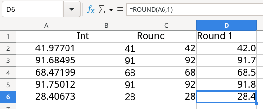
Table lookups

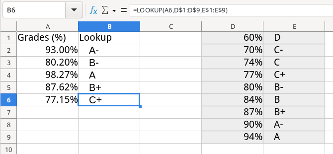
The table lookup feature in spreadsheets is a huge time-saver. Tables can make it easy to transform one value into another, depending on values stored in columns or rows.

I use vertical lookups to calculate final grades when I teach classes. I start by defining a lookup table, with the data sorted in ascending order. In the first column, I give the “bottom” value of each grade level, such as 0% for F, 60% for D, 70% for C, 80% for B, and 90% for A. In the second column, I list the corresponding letter grade.

To find values with VLOOKUP, give the value to locate in the table, then the range for the full table, and the column (counting from 1 for the first column in the table) that holds the result that you want to return from the lookup. If your data is sorted in the table, also give a TRUE value as the fourth option.

For example, here is a sample gradebook calculation that looks up the letter grade for five students:

A shortcut to vertical lookups is the LOOKUP function. To look up values with this simpler function, give the value to locate in the sorted table, then the range of the first column (the column with the number values) and the range of the second column (the column with the result).

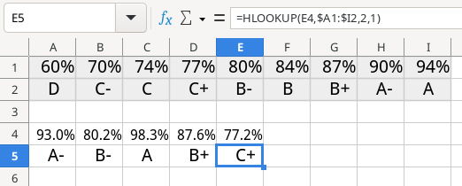
If your data is in columns instead of rows, you can use the HLOOKUP function to do a horizontal lookup. The usage is otherwise the same as VLOOKUP: start with the value to find in the table, then the range of the full table, and the column number with the result. If the data is sorted in the table, give a TRUE value in the fourth option.

Let the spreadsheet do the work

Spreadsheets are an invaluable tool to work with data. Don’t worry about memorizing every possible function in the spreadsheet; most people tend to stick to a few functions that help them get their work done. I find these 17 functions will help me tackle most data that I need to work with.

Use this as a starting point to explore the other spreadsheet functions available in LibreOffice Calc. Tap the F1 key in LibreOffice Calc to enter the Help system, and click on the link to list functions by category. Or visit the Functions by Category page on the LibreOffice.org website for a full reference.